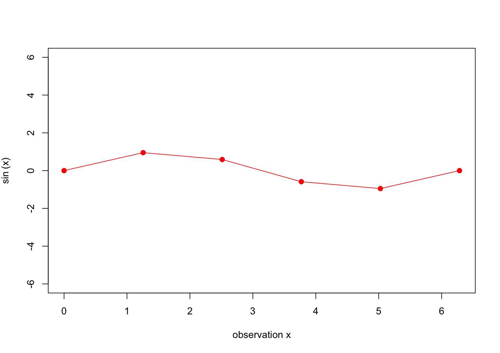
Figure 1: seven observation \((x_i,y_i), i = 1,2,\dots,6\).
Our objective is to model this data using the GP framework. We now introduce notations used through the note before diving into the main concept. We adopt notations from Garnett1. A GP on \(f\) is defined as follows \[
p(f) = GP(f; \mu, K),
\tag{1}\] where \(\mu: \mathcal{X} \to \mathbb{R}\) and \(K: \mathcal{X\times X}\to \mathbb{R}\) are a mean function and positive semidefinte covariance function (or kernel). Also, let’s \(\phi = f(x)\) corresponding to the observed datum \(x\). Thus,
1. Garnett R. Bayesian optimization. Cambridge University Press; 2023.
This setting can also be described using the multivariate normal distribution; thus, \[
p(\boldsymbol\phi) = \mathcal{N}(\boldsymbol\phi; \boldsymbol\mu, \boldsymbol\Sigma),
\] where \(\boldsymbol\mu = \mathbb{E}(\boldsymbol\phi|\boldsymbol x) = \mu(\boldsymbol x)\) and \(\boldsymbol\Sigma = \text{cov}(\boldsymbol\phi|\boldsymbol x) = K(\boldsymbol{x}, \boldsymbol{x})\).
set.seed(111)n =100x_pr =matrix(seq(-0.5, 2*pi+0.5, length=100), ncol=1)d_pr =distance(x_pr)K_pr =exp(-d_pr)mu_pr =numeric(length(x_pr))|>as.matrix()y_pr = mvtnorm::rmvnorm(3, mu_pr, K_pr)matplot(x_pr, t(y_pr), type ="l", lty =1, xlab ="prior x", ylab ="density", ylim =c(-6,6), col =c("blue","green", "gray"))points(x_obs, y_obs, pch =16, cex =1.2, type ="o", col ="red" )
Figure 2: Prior Gaussian.
Having used this familiar notations, the conditional normal distribution is obtained with ease based on the standard formulae of conditional multivariate normal distribution. Consider the following GP \[
p(f,\boldsymbol y) = \mathcal{GP}\bigg(
\begin{bmatrix}
f \\
\boldsymbol y
\end{bmatrix};
\begin{bmatrix}
\mu \\
\boldsymbol m
\end{bmatrix},
\begin{bmatrix}
K & \kappa^{\top} \\
\kappa & \boldsymbol C
\end{bmatrix}
\bigg),
\] which implies that \(\boldsymbol y \sim \mathcal{N}(\boldsymbol y; \boldsymbol m, \boldsymbol C)\) and \(\kappa(x) = \text{cov}(\boldsymbol y, \phi|x)\). Let \(D \equiv \boldsymbol y\) is the observed data and, thus, the conditional GP is \[
\begin{aligned}
&p(f|D) = \mathcal{GP}(f; \mu_D, K_D),\\
\text{ where } \\
&\mu_D(x) = \mu(x) + \kappa(x)^{\top}\boldsymbol{C}^{-1}(\boldsymbol y - \boldsymbol m) \\
&K_D(x,x_*) = K(x,x_*) - \kappa(x)^{\top}\boldsymbol{C}^{-1}\kappa(x_*)
\end{aligned},
\tag{2}\] without loss of generality, we can assume \(\boldsymbol\mu = \boldsymbol m = \boldsymbol 0\).
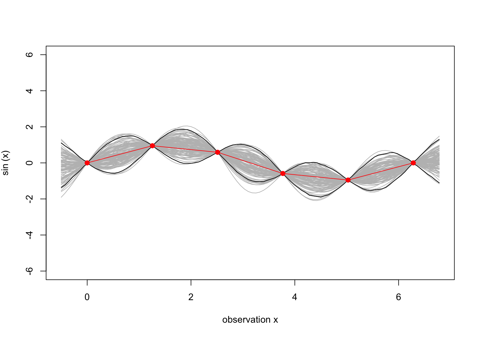
The above setting is the brief summary of the GP. We now specify the conditional GP whose prior is shown in Figure 2 and the observed data \(D\) is shown in Figure 1. Note that the covariance matrix is calculated using the squared exponential, i.e. \(K(x,x_*) = \exp\{-(x-x_*)^2\}\).
d_obs =distance(x_obs)C_obs =exp(-d_obs)kap =distance(x_pr, x_obs)|> {\(i) exp(-i)}()mu_D = mu_pr + kap%*%solve(C_obs)%*%(y_obs)K_D = K_pr - kap%*%solve(C_obs)%*%t(kap)y_pos = mvtnorm::rmvnorm(10000, mu_D, K_D)|>t()ci =apply(y_pos,1, HDInterval::hdi)matplot(x_pr, t(ci), type ="l", col ="black", lty =1, ylim =c(-6,6), xlab ="observation x", ylab =expression(sin~"(x)" ) )for(i in1:100) lines(x_pr, y_pos[,i], col ="gray")matplot(x_pr, t(ci), col ="black", lty =1, add = T, type ="l")#lines(x, m )lines(x_obs, y_obs, pch =16, col ="red", type ="o", cex =1.2)
Figure 3: The predictive surface interpolates the data.
2 GP with hyperparameters
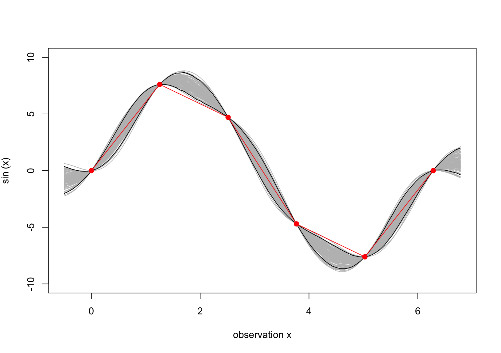
Why do we need to consider the hyperparamters in GP? Let’s consider a scenario where the true distribution of the data has a large variance compared to the prior fitted.
y_obs_new = y_obs*8mu_D_new = mu_pr + kap%*%solve(C_obs)%*%(y_obs_new)K_D_new = K_pr - kap%*%solve(C_obs)%*%t(kap)set.seed(1)y_pos = mvtnorm::rmvnorm(10000, mu_D_new, K_D_new)|>t()ci =apply(y_pos,1, HDInterval::hdi)matplot(x_pr, t(ci), type ="l", col ="black", lty =1, ylim =c(-10,10), xlab ="observation x", ylab =expression(sin~"(x)" ) )for(i in1:100) lines(x_pr, y_pos[,i], col ="gray")matplot(x_pr, t(ci), col ="black", lty =1, add = T, type ="l")#lines(x, m )lines(x_obs, y_obs_new, pch =16, col ="red", type ="o", cex =1.2)
Figure 4: The predictive surface interpolates the data as the scale of 8 is added.
Compared to Figure 3, the uncertainty about the true function (red line) is lower, which is our desire, but the corresponding credible intervals do not capture the true function. Thus, we need to adjust the covariance \(\boldsymbol C\), i.e.
\[
p(\boldsymbol y) = \mathcal{N}(\boldsymbol y; \mu, \tau^2\boldsymbol C),
\] which is analogous to defining \(f_* = \tau f\).
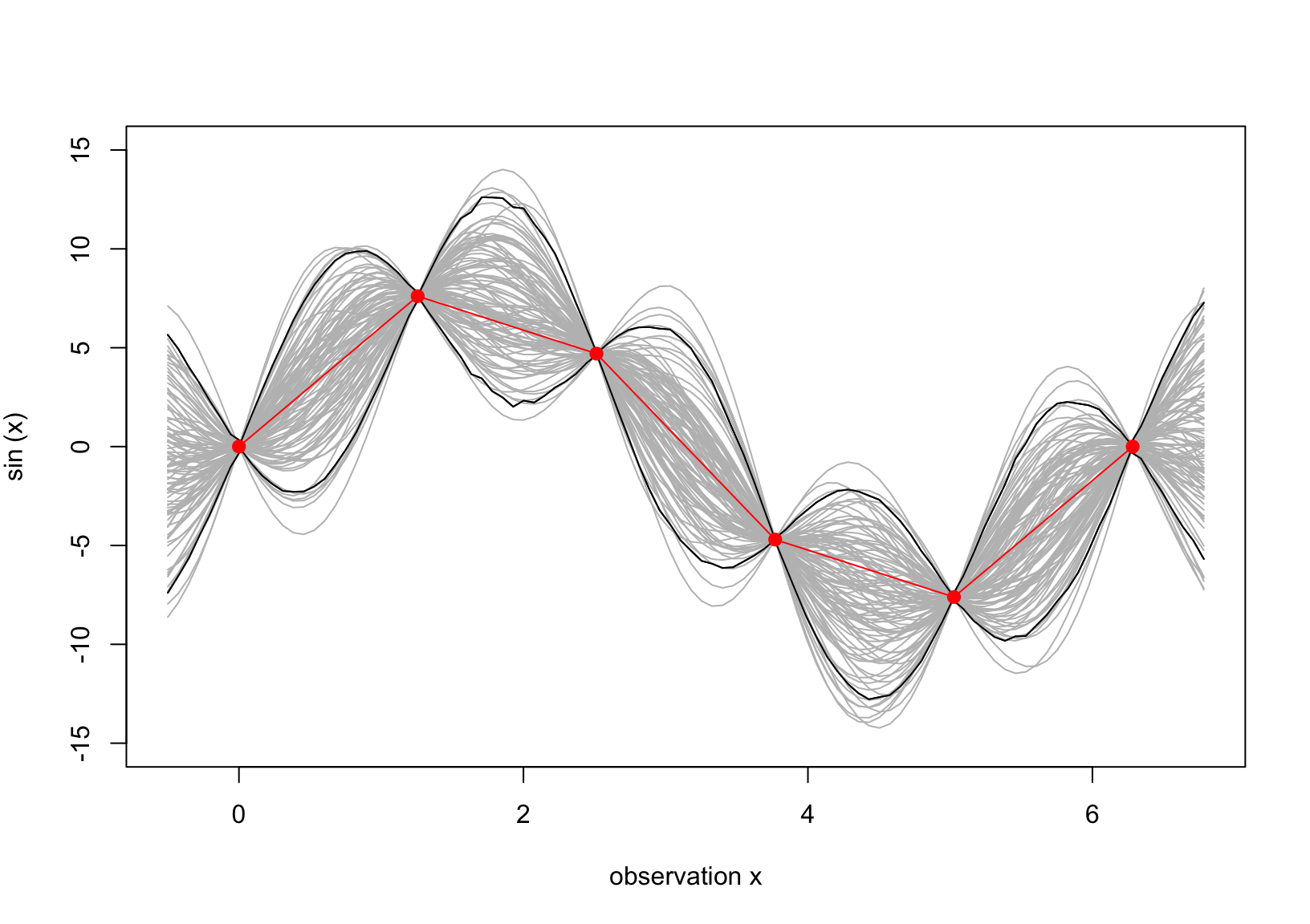
We then can calculate the maximum likelihood estimator of \(\tau^2\) as follows \[
\hat\tau^2_{ML} = \frac{\boldsymbol y^{\top}\boldsymbol\Sigma^{-1}\boldsymbol y}{\text{length}(\boldsymbol y)},
\] detail can be found in Gramacy et al.2 We now plug-in \(\hat\tau^2_{ML}\) into Equation 2. Technically, this leads to multivariate student-\(t\) distribution, but we assume that the degree of freedom is large enough to approximate the \(t\) using the normal distribution.2. The mean \(\mu_D\) remains unchanged, but the covariance matrix changes to the following form: \[
K_D(x,x_*) = \big[K(x,x_*) - \kappa(x)^{\top}\boldsymbol{C}^{-1}\kappa(x_*)\big]\hat\tau^2_{ML},
\tag{3}\] which can be deduced from the new setting \(f_*:x \to \tau f(x)\), i.e. \[
\text{cov}[\tau f|\tau] = \tau^2K.
\]
2. Gramacy RB. Surrogates: Gaussian process modeling, design, and optimization for the applied sciences. Chapman; Hall/CRC; 2020.
It is worth noting that the the MLE of \(\tau\) is a function of \(f\) which indicates that the observed data are now involved in the uncertainty, compared to the formula in Figure 2.
tau2hat<-drop(t(y_obs_new)%*%C_obs%*%y_obs_new/length(y_obs_new))K_D_new_up = tau2hat*K_D_new####set.seed(1)y_pos = mvtnorm::rmvnorm(10000, mu_D_new, K_D_new_up)|>t()ci =apply(y_pos,1, HDInterval::hdi)matplot(x_pr, t(ci), type ="l", col ="black", lty =1, ylim =c(-15,15), xlab ="observation x", ylab =expression(sin~"(x)" ) )for(i in1:100) lines(x_pr, y_pos[,i], col ="gray")matplot(x_pr, t(ci), col ="black", lty =1, add = T, type ="l")#lines(x, m )lines(x_obs, y_obs_new, pch =16, col ="red", type ="o", cex =1.2)
Figure 5: The predictive surface of the scale-adjusted GP.