A Simulation Study to Validate Joint Models for Longitudinal and Survival Data
Agenda
- Introduction
- Model
- Simulation
- Results
- Conclusion
Introduction
Study Context
- Patients with chronic kidney disease are monitored over time
- Regular measurements of serum creatinine reflect kidney function
- Lower creatinine values indicate better kidney function
Outcomes of Interest
- Longitudinal outcome: Serum creatinine (continuous, time-varying)
- Survival outcome: Time to kidney failure or initiation of dialysis
Introduction
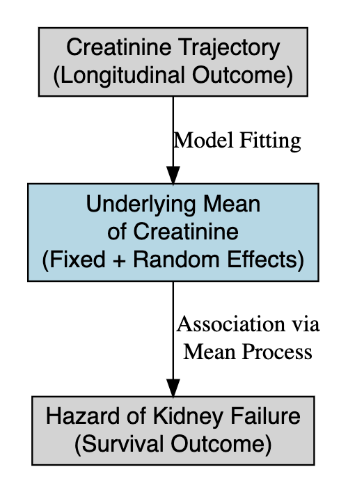
Joint Modeling Solution
- Link the true underlying creatinine trajectory (fixed + random effects) to the hazard of kidney failure.
- Account for patient-specific progression of creatinine.
- Incorporate uncertainty and allow dynamic prediction of event risk.
- Naturally integrate Bayesian priors for clinical knowledge.
Challenges
- Creatinine trajectory is strongly linked to the risk of kidney failure
- Measurement error and individual heterogeneity complicate analysis
- Separate models for each process may yield biased survival estimates
Joint models
Longitudinal model
\[ \begin{aligned} y_{ij} &= \boldsymbol{x_{i}'\beta} + \boldsymbol{z_i'b}+\epsilon_{ij}\\ &= m_i(t) + \epsilon_{ij} \end{aligned} \]
Survival model
\[ h_i(t) = h_0(t)\exp{\{\alpha_2m_i(t) + \boldsymbol{k_i'\alpha_1}\}} \]
Joint models
Longitudinal submodel
\[ \begin{aligned} y_{ij} &= \beta_0 + \beta_1\mathrm{treatment}_i + b_{0i} + b_{1i}\mathrm{time}_{ij} + \epsilon_{ij}\\ &= m_i(t) + \epsilon_{ij} \end{aligned} \] Survival submodel
\[ h_i(t) = h_0(t)\exp\{\alpha_2m_i(t) + \alpha_1\mathrm{treatment}_i\} \]
- \(\beta_0\) and \(\beta_1\) are fixed intercept and effect of the treatment on longitudinal outcome.
- \(b_{0i}\) and \(b_{1i}\) are random effect associated with subject \(i\).
- \(\alpha_2\) is the fixed effect associated with \(m_i(t)\).
- \(\alpha_1\) is the fixed effect of treament on event time.
Joint models
\[ \begin{aligned} &y_{ij} = \beta_0 + \beta_1\mathrm{treatment}_i + b_{0i} + b_{1i}\mathrm{time}_{ij} + \epsilon_{ij} = m_i(t) + \epsilon_{ij}\\ &h_i(t) = h_0(t)\exp\{\alpha_2m_i(t) + \alpha_1\mathrm{treatment}_i\} \end{aligned} \]
The joint model assumes:
- Treatment does not change over time.
- Longitudinal outcome is a linear function of time.
- Treatment has both direct and indirect effect on event time.
- The total treatment effect is \(\beta_1\alpha_2 + \alpha_1\).
Model
We fit the joint model using the Bayesian framework, which is completed after defining prior distributions, a priori information about parameters before observing data.
Longitudinal submodel
\[ \begin{aligned} &\{\beta_k\}_{k=1}^2 \sim N(0, 10), \quad b_{0i} \sim N(0,10), \quad b_{1i}\sim U(0,4) \\ &\epsilon_{ij} \sim N(0,\sigma^2), \quad \sigma \sim N^+(0,5) \end{aligned} \]
Survival submodel
We use the gamma process with group-data likelihood, as it is the most commonly used nonparametric prior process for the Cox model.
Model
Survival submodel
Under the Cox model, the joint probability of survival of \(n\) subjects is
\[ \begin{aligned} &P(\boldsymbol Y > \boldsymbol y|\boldsymbol\alpha,X,H_0) = \exp\bigg\{-\sum_{j=1}^n \exp(\boldsymbol x_j'\boldsymbol\alpha)H_0(y_j) \bigg\}\\ &H_0 \sim \mathrm{GammaProcess}(c_0H^*, c_0), \end{aligned} \]
Under assumption of exponential distribution, we have \(H^*(y) = \gamma_0y\). Thus,
\[ h_j = H_0(s_j) - H_0(s_{j-1}) \sim Gam(\kappa_{0j}-\kappa_{0,j-1},c_0), \] where \(\kappa_{0j} = c_0H^*(s_j)\). I.e
\[ h_j \sim Ga(c_0\gamma_0(s_j-s_{j-1}), c_0) \] \(c_0\) and \(\gamma_0\) are hyper-parameters, and \(0 < s_1 < s_2 < \dots < s_J\) with \(s_J > y_i \forall i\).
Model
Survival submodel
Thus, the likelihood function is
\[ L(\boldsymbol\alpha, \boldsymbol h|D) \propto \prod_{j=1}^JG_j, \] where \(\boldsymbol h = (h_1,\dots,h_J)'\) and
\[ G_j = \exp\bigg\{-h_j\sum_{k \in \mathfrak R_j -\mathfrak D_j}\exp\boldsymbol x'\boldsymbol\alpha \bigg\}\prod_{l \in \mathfrak D_j}\bigg[1 - \exp\{-h_j\exp(\boldsymbol x'\boldsymbol\alpha)\}\bigg] \]
Since \(H_0\) enters the likelihood only through the \(h_j\)’s, parameters in the likelihood are \((\boldsymbol\alpha,\boldsymbol h)\).
Model
Survival submodel
We set
\[ \begin{aligned} &\alpha_1 \sim N(0,10), \quad \alpha_2 \sim N(0,3)\\ & \gamma_0 = 0.1,\quad c_0 = 0.01\quad \text{(suggested by Ibrahim et al.)} \end{aligned} \]
Model
Since the longitudinal and survival time are conditional independent given random effect, the complete data log-likelihood is
\[ l(\boldsymbol\theta) = \sum_{i=1}^n\ln\big\{\phi(y^{(longitudinal)}_i|\boldsymbol{b_i,\beta},\sigma^2) \phi(\boldsymbol b_i|\Sigma_b) \phi(y^{(survival)}_i|\boldsymbol b_i, \boldsymbol\beta, \boldsymbol\alpha) \big\}, \] where \(\phi(.|.)\) denotes the appropriate normal probability density function.
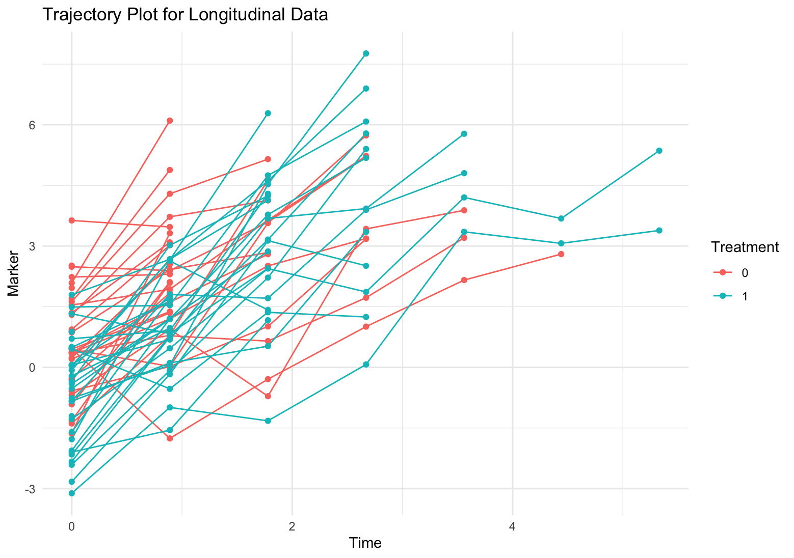
Data simulation
\[ \begin{aligned} &y_{ij} = \beta_0 + \beta_1\mathrm{treatment}_i + b_{0i} + b_{1i}\mathrm{time}_{ij} + \epsilon_{ij} = m_i(t) + \epsilon_{ij}\\ &h_i(t) = h_0(t)\exp\{\alpha_2m_i(t) + \alpha_1\mathrm{treatment}_i\} \end{aligned} \]
- Recall that \(y_{ij}\) is a linear function of time.
- Thus, \(m(t)\) is also a linear function of time.
- We adapt the method proposed by Austin to generate the survival time with time-varying covariates under two assumptions
- Survival time follows exponential distribution.
- The time-varying covariate is a linear function of time.
\[ T = \ln\bigg[\frac{\alpha_2\beta_2(-\ln u)}{\lambda\exp\{\alpha_2k+\alpha_1\mathrm{treatment}\}}+1\bigg]\frac{1}{\alpha_2\beta_2}, \] where \(u \sim \mathrm{Uniform}(0,1)\).
Data simulation
- First, we simulate survival time for each subject.
- Second, we simulate the longitudinal observations for each subject.
- Third, we remove all longitudinal observations with time beyond survival time.
- Lastly, define censors: the event times beyond the 60% quantile are set to censor time.
We simulate 4 scenarios using different number of subjects and intervals.
- 30 subjects per arm + 9 intervals (10 time pints).
- 30 subjects per arm + 59 intervals (60 time points).
- 60 subjects per arm + 59 intervals (60 time points).
- 60 subjects per arm + 99 intervals (100 time points).
Data simulation
We simulate data using the same setting of fixed and random parameters.
\[ \begin{aligned} &\beta_0 = 0.5,\quad \beta_1 = -1.2, \quad \lambda = 0.05 \\ &b_0 \sim N(0,1), \quad b_1 \sim U(1,3), \quad \epsilon \sim N(0,1)\\ &\alpha_2 = 0.8, \quad \alpha_1 = -0.5 \end{aligned} \]
- Treatment decreases the longitudinal outcome (i.e. serum creatinine, which improves the kidney function.)
- The kidney function is worse over time.
- As longitudinal outcome (serum creatinine) decreases, the hazard decrease.
- Treatment also decreases hazard.
Model fitting
- All models are fitted using
stanin the R environment. stanemploys full Bayesian inference via Hamiltonian Monte Carlo.- We generate 3000 samples after 4000 warm-up iterations.
- Model convergence is assessed using \(\hat{R}\), with values below 1.1 indicating convergence.
Results
We report summaries (mean and 95% highest density posterior intervals (HDI)) of primary parameters:
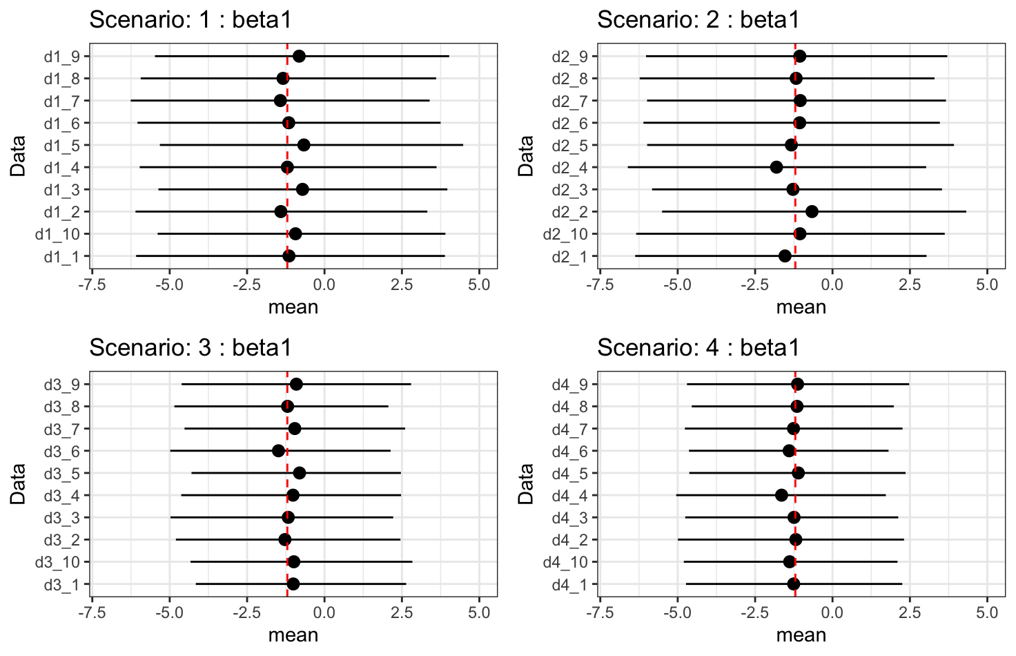
- \(\beta_1\): treatment effect on longitudinal outcome.
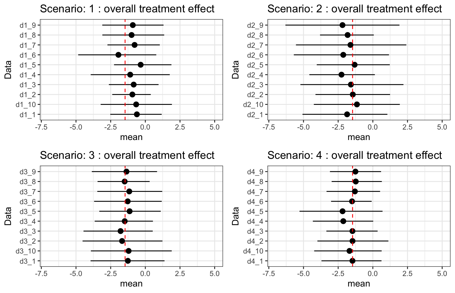
- \(\beta_1\times\alpha_2 + \alpha_1\): overall treatment effect on hazard.
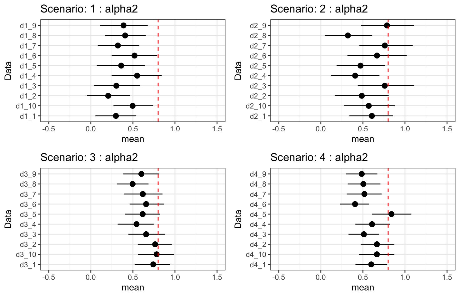
- \(\alpha_2\): indirect treatment effect on hazard.
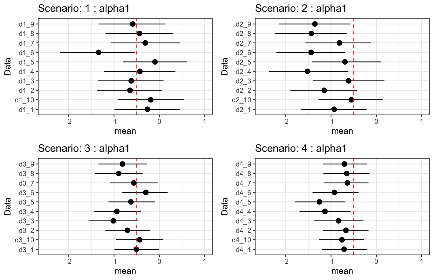
- \(\alpha_1\): direct treatment effect on hazard.
Results - \(\beta_1\): treatment effect
Results - \(\beta_1\times\alpha_2 + \alpha_1\): overall treatment effect
Results - \(\alpha_2\): indirect treatment effect
Results - \(\alpha_1\): direct treatment effect
Discussion
- Treatment effect on longitudinal outcomes is fully recovered.
- Overall treatment effect on hazard is fully recovered.
- Indirect treatment effect is under-fitting. Increasing longitudinal observations may improve, but it does not guarantee we can fully recover the true effect.
- Increasing the number of subjects improves uncertainty.
Discussion
- As the indirect treatment effect improves, the estimate of the direct treatment effect worsens. This is due to collinearity between \(\alpha_1\) and \(\alpha_2\beta_1\).
- The model may “choose” a lower value for \(\alpha_2\) so that, when combined with \(\beta_1\), it doesn’t overstate the total effect of treatment.
- The data might only provide enough information to identify the combined effect \(\alpha_1 + \alpha_2\beta_1\), not the two parts separately.
- This means that the specific contribution of treatment via the indirect effect combines with the direct treatment effect in a way that the survival likelihood only “sees” \(\alpha_1 + \alpha_2\beta_1\).
- Forcing the model to recover a higher \(\alpha_2\) makes \(\alpha_1\) become under-fitting since the model is trying to split a fixed overall effect into two highly correlated components subject to the overall treatment effect.